iqgen: Spatial RF Synthesis, Antennas & Spectrum Analysis
A useful RF simulator has to preserve more than a recognizable spectrum. Symbols, oscillator phase, propagation delay, and recording time must remain consistent as GPU work is divided into frames. iqgen tackles that problem by generating a continuous sampled RF environment, while a separate waterfall process receives, analyzes, and records its output.
This is part of tsim. The portable compute path uses WGFX’s SDL3 GPU and Slang architecture; native CUDA and ROCm/HIP backends provide another execution path for supported workloads.

From Emitters to Samples
The generator starts each frame with receiver thermal noise, adds the enabled emitters, and packs the resulting complex samples for publication. That sequence hides several different kinds of state:
graph LR
    sources["Audio, files, PRBS"] --> waveform["Waveform synthesis"]
    waveform --> effects["Shaping, PA, RF impairments"]
    geometry["Positions, paths, antenna gain"] --> channel["Delayed and scaled path contributions"]
    effects --> channel
    channel --> mix["Receiver IQ + thermal noise"]
    mix --> pack["Pack Float32 / Int16 / Int12 / Int8"]
    pack --> shm["GPU readback + msg shared ring"]
    shm --> viewer["FFT windows, waterfall, SigMF"]
Payload offsets, carrier phase, OFDM symbol positions, and filter history advance across frames. Otherwise, a frame boundary would become a periodic discontinuity in the waveform. Source ingestion runs separately from sample generation: audio capture and file playback supply AM/FM inputs, while binary files and deterministic PRBS sequences supply digital symbols.
This distinction also matters when a source pauses. A pause in a burst should produce quiet samples at the proper sample times, rather than making the receiver’s time axis jump forward.
Waveform Fidelity
CW and noise are useful baseline signals, but digital modulation reveals whether the sampled implementation behaves consistently. PSK/QAM uses Gray mapping, and its polyphase root-raised-cosine filter shapes transitions between symbols. An explicit symbol rate can be set independently of the sample rate; rolloff controls the excess bandwidth of the shaped signal.
OFDM adds a different set of boundaries. The useful symbol contains carriers allocated to data, pilots, guard regions, and optionally a nulled DC bin. A cyclic prefix repeats the end of that symbol, while windowing softens its edges. Power-of-two carrier configurations can use an IFFT-based table path; custom configurations also have direct-sum implementations. Native backends choose between the implementations according to the carrier configuration.
The practical controls answer different questions:
| Control | What it changes |
|---|---|
| Symbol rate and RRC rolloff | Digital timing and occupied single-carrier bandwidth |
| OFDM guards and DC null | Which carriers are active |
| Pilots | Known carrier values within the OFDM signal |
| Cyclic prefix | Repeated samples available to accommodate channel delay spread |
| Window rolloff | The transition at OFDM symbol boundaries |
| Payload scrambling | Repeatable whitening of otherwise repetitive payload bits |
Pulsed signals and ASR-9/ASR-11 presets add PRF, pulse width, and rotating-beam amplitude modulation. Link16-like FHSS provides deterministic hopping and sparse slot activity. These profiles reproduce public waveform traits for RF testing and visualization; they do not implement operational Link 16 messaging, protected hopsets, or interoperable timing.
The Receiver Has a Location
Both emitters and receivers have WGS-84 geodetic and double-precision ECEF positions. The selected coordinate format determines which representation is authoritative on input; API responses include both. Path loss uses three-dimensional slant range, and rotating radar bearing derives from the same geometry.
Directional gain adds another transformation. A ray first has a direction in the local true-north/horizon frame, then moves into the antenna’s mounted frame. Physical yaw, pitch, and roll describe the mount; electrical azimuth/elevation steering describes where the array points within that frame. Keeping those separate makes it possible to rotate a platform without accidentally redefining its beam steering.
The channel supports direct-only, manual tapped-delay, two-ray-ground, and stochastic tapped-delay models. A manual echo has excess delay, relative gain, phase, and Doppler. Delay can be fractional in sample units, and phase continuity must survive the next frame. A multipath delay of one microsecond is one sample at 1 MS/s but one thousand samples at 1 GS/s, so the same physical channel has very different history-storage requirements at different rates.
Path diagnostics expose lengths, delays, gains, directions, and estimated channel characteristics. Those are useful for distinguishing weak reception caused by geometry from a waveform or tuner configuration error.
Antenna Patterns as Computed Data
The companion antenna tool sums coherent complex fields from array elements and simultaneous beams. Interference therefore appears in the resulting pattern, including sidelobes and grating lobes. Rectangular, hexagonal, circular, linear, and sparse geometries share this approach; analytical dish, horn, dipole, and other models have their own patterns.
Overlapped beams divide the aperture’s power among beams. Strip subarrays use a smaller effective aperture for each beam. Interleaving preserves aperture extent while increasing effective spacing, which can introduce grating lobes. Tapering and phase errors alter the computed pattern rather than just a displayed gain number.

The hexagonal array offers another view of how geometry and a partitioned aperture shape the resulting lobes.

The spherical tab turns full-coverage gain samples into GPU color, displacement, and normal maps. Orbiting the view does not require recomputing the pattern. Its radius can show dB, linear amplitude, or linear power: a dB radius intentionally compresses large differences, while linear power makes steering loss much more obvious. Optional backlobes use a configurable front-to-back ratio.
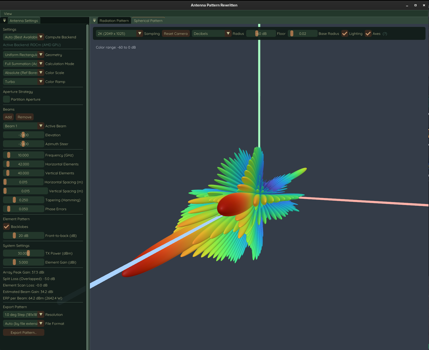
High-resolution geometry has a real cost. The documented 4K spherical grid contains approximately 8.4 million vertices and 16.8 million triangles, with roughly 770 MiB of GPU mesh and material data before temporary upload storage. It is a detailed inspection mode, not a free increase in visual quality.
Moving IQ Between Processes
Local streaming defaults to shm;none;iqgen, backed by msg. Each application block contains a 48-byte versioned header with format, UTC timestamp, sample rate, usable bandwidth, and center frequency. Large frames split into sample-aligned blocks, and a late listener learns the tuning metadata from its next block.
The output supports Float32, Int16, dense Int12, and Int8 complex samples. Int16 is the default. At 1 GS/s, a pair of 16-bit I/Q values consumes 4 GB/s, or 32 Gb/s, before headers. Compression is not part of this local packed-IQ path.
The copy boundaries are explicit: GPU samples are read back to host memory, packed bytes copy into the shared ring, and each receiver copies into its bounded reservoir. Shared memory removes local UDP packet and socket overhead, but the application still pays for readback and buffering. If a reservoir fills, its reader holds up publication; a send can time out and throw. Additional listeners share ring storage but keep their own reservoirs and processing costs.
Use separate channel names for independent generators. An IP:PORT endpoint selects VITA-49 UDP when the receiver is across the network.
Spectrum Resolution and Waterfall Time
A display does not need to convert every received sample into a plotted pixel. The current viewer walks timestamp-ordered packed payloads and converts selected FFT windows. All received samples advance the row clock; samples outside the selected windows are omitted from analysis without becoming receive gaps. Recording continues to consume contiguous IQ.
Frequency spacing follows sample rate / FFT length. For a 4096-sample window, 1 GS/s gives approximately 244 kHz bin spacing, while 2.5 MS/s gives approximately 610 Hz. Zooming therefore needs frequency translation and anti-alias filtering to analyze a narrower band at a reduced effective rate. GPU conversion and cascaded half-band stages provide that path.
Waterfall row duration follows sample time rather than display frames. At 10 ms per row, 1024 rows represent 10.24 seconds. Averaging multiple windows combines linear power within a row; it does not change the row’s duration. At very narrow zooms, the effective interval can extend to fit an FFT window.
This separates three clocks: sample generation, analysis rows, and screen refresh. A 144 Hz UI is not evidence that the generator is keeping up, so telemetry reports receive traffic, rows, skipped viewer samples, and generator underruns separately.
Measurements and Their Scope
October 10 measurements on a Ryzen 9 7950X / Radeon RX 9070 XT Linux host tested the integrated CPU payload generator, shared ring, and receive reservoir with 32 GiB cases:
| Validation | Delivered GB/s | Receive drops |
|---|---|---|
| Sample checks | 11.77 | 0 |
| Every payload byte | 5.26 | 0 |
| Sample checks, paced at 4 GB/s | 4.00 | 0 |
A separate 20-second nine-signal run at 800 MHz usable bandwidth, 1 GS/s, and Int16 output delivered about 32 Gb/s after startup. The viewer generally ran near 144 Hz with zero reported skipped samples. Startup produced six underruns; subsequent reporting intervals produced zero. These were short live checks, not long interactive soaks. The measurement file records the benchmark and GUI scopes separately.
Running and Inspecting the Pipeline
After the tsim build, start the programs in separate terminals from the repository root:
./build/dist/bin/iqgen/iqgen --iq "shm;none;iqgen" --api-port 3000
./build/dist/bin/iqgen/waterfall --iq-listen "shm;none;iqgen" --api-url http://127.0.0.1:3000
The installed build/dist/bin/iqgen/ directory also has a Process Compose group. On Linux/macOS, process-compose -U starts the pair and waits for the backend API before launching the viewer. Backend state changes propagate to connected frontends through WebSockets.
Start with a CW tone to inspect frequency and gain, then introduce shaping, an echo, or an impairment individually. GeoJSON/KML scenario export can put the receiver and emitters into tview without starting generation. The IQ guide documents controls and native-backend coverage; the antenna guide explains pattern scaling and geometry costs.
For packet acquisition and delivery rather than waveform inspection, continue with multi-radio communication. For the whole suite, return to the tsim overview.